---
title: "Background: Toy Models of Superposition"
subtitle: "The petri dish the essay is arguing with, reproduced, plus the essay's own modification of it"
---
Before reading the essay's "Superposition" section it helps to have run the toy model that
made superposition a precise idea: Elhage et al., [*Toy Models of
Superposition*](https://transformer-circuits.pub/2022/toy_model/index.html) (Anthropic, 2022).
The essay's appendix calls it "careful work, the kind our field should aspire to" and says it
found no problems with its experiments. Its objection is to the *framing*: the toy prices the
cost of sharing a neuron (interference) but not the benefit (reuse by downstream readers),
because in the toy nothing is downstream.
This page does three things. It reproduces the toy's main results in a few seconds of CPU
time, it reproduces the essay's modification (correlated inputs plus a layer of hidden
neurons), and it states what we should carry forward into the essay proper.
## 1. The setup
There are $n$ **features**, collected in a vector $x \in [0,1]^n$. Feature $i$ is present with
probability $1-S$, with amplitude uniform on $[0,1]$, and absent (exactly zero) otherwise. $S$
is the **sparsity**. The network must squeeze $x$ through a bottleneck of width $m < n$ and
recover it:
$$
h = W x \in \mathbb{R}^m, \qquad \hat x = \mathrm{ReLU}(W^{\mathsf T} h + b).
$$
The loss is a weighted reconstruction error $\sum_i I_i\,(x_i - \hat x_i)^2$ with
**importances** $I_i = 0.9^i$, so earlier features matter more. The whole model is the
$m \times n$ matrix $W$ and the bias $b$. Column $W_i \in \mathbb{R}^m$ is the direction in
the bottleneck that feature $i$ is written to and read from.
Why ReLU on the output matters: with a linear decoder the best the model can do is PCA, keeping
the top $m$ features and dropping the rest. ReLU lets it do better, because small
interference from other features can be clipped off at zero if the interfering features are
usually absent. That is the whole mechanism of superposition: *sparsity makes interference
cheap*.
The diagnostics used below, all computable from $W$:
- $\|W_i\|$: how strongly feature $i$ is represented at all (0 means dropped).
- The **superposition index** $\sum_{j\ne i} (\hat W_i\cdot W_j)^2$: how much other features
overlap with feature $i$'s direction. Zero means a private direction.
- The **dimensionality** $D_i = \|W_i\|^2 / \sum_j (\hat W_i\cdot W_j)^2$. A feature with its
own orthogonal direction has $D_i = 1$; two features sharing a direction antipodally have
$D_i = \tfrac12$; the paper shows the values cluster at simple fractions.
```{python}
#| code-summary: "Imports and helpers"
import sys, pathlib
sys.path.insert(0, str(pathlib.Path.cwd().parent))
import numpy as np, torch, matplotlib.pyplot as plt
from common.toy_models import (TMS, TMSHidden, train, sample_independent, sample_grouped,
                               feature_norms, superposition_index, feature_dimensionality,
                               cosine_matrix)
plt.rcParams.update({"figure.dpi": 110, "font.size": 9})

def fit_tms(n, m, S, steps=4000, seed=0, importance_decay=0.9):
    gen = torch.Generator().manual_seed(seed)
    model = TMS(n, m, gen)
    imp = torch.tensor([importance_decay**i for i in range(n)])
    sampler = lambda b, g: sample_independent(b, n, S, g)
    train(model, sampler, imp, steps=steps, seed=seed)
    return model
```
## 2. From "keep the top $m$" to packing, as sparsity rises
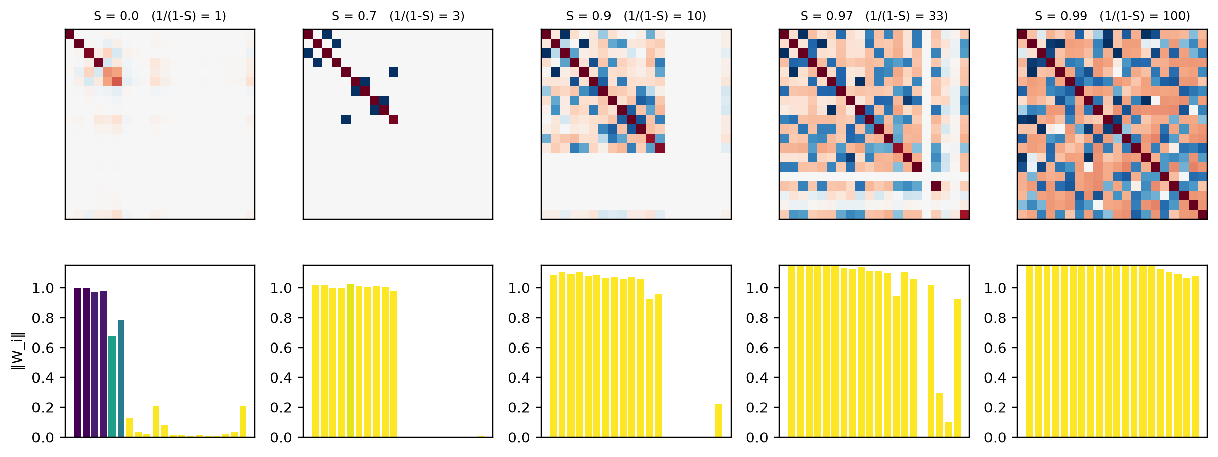
The paper's headline figure: $n=20$ features in $m=5$ dimensions, trained at increasing
sparsity. Each panel shows the Gram matrix $W^{\mathsf T}W$ (which features overlap with
which) and, below it, each feature's norm coloured by its superposition index.
```{python}
#| code-summary: "Train n=20, m=5 across sparsity"
#| fig-cap: "Top row: $W^{\\mathsf T}W$. Bottom row: $\\|W_i\\|$ per feature, coloured by superposition index (dark = private direction, yellow = heavily shared). At $S=0$ the model keeps the five most important features and drops the rest. As features become rarer it represents more of them, first in antipodal pairs, then in denser arrangements."
n, m = 20, 5
sparsities = [0.0, 0.7, 0.9, 0.97, 0.99]
models = {S: fit_tms(n, m, S, steps=8000) for S in sparsities}

fig, axes = plt.subplots(2, len(sparsities), figsize=(2.2*len(sparsities), 4.6),
                         gridspec_kw={"height_ratios": [3, 1.6]})
for j, S in enumerate(sparsities):
    W = models[S].W.detach()
    G = (W.T @ W).numpy()
    ax = axes[0, j]
    ax.imshow(G, cmap="RdBu_r", vmin=-1, vmax=1)
    ax.set_title(f"S = {S}   (1/(1-S) = {1/(1-S):.0f})", fontsize=8)
    ax.set_xticks([]); ax.set_yticks([])
    ax = axes[1, j]
    norms = feature_norms(W); sup = superposition_index(W)
    ax.bar(range(n), norms, color=plt.cm.viridis(np.clip(sup, 0, 1)))
    ax.set_ylim(0, 1.15); ax.set_xticks([]);
    if j == 0: ax.set_ylabel("‖W_i‖")
plt.tight_layout()
```
Reading the figure. With dense features ($S=0$) every feature is on almost every time, so any
overlap is paid for on every sample; the model keeps the five most important features on
orthogonal axes and drops the other fifteen. As features become rare, the expected cost of
interference falls like $(1-S)$ while the benefit of representing an extra feature does not,
so more and more features are packed in. The first packing is **antipodal pairs** (two
features on the same axis with opposite sign: the ReLU separates them because they are
rarely both present), then denser polytopes.
## 3. The geometry of packing
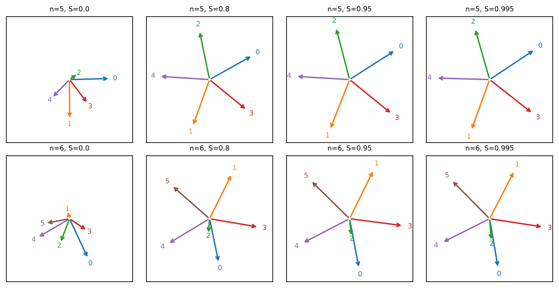
With $m = 2$ we can draw the columns $W_i$ directly.
```{python}
#| code-summary: "Train n=5 and n=6 features into m=2 dims at high sparsity"
#| fig-cap: "Feature directions $W_i$ in a two-dimensional bottleneck. At low sparsity only two features survive. At high sparsity the model spreads all of them around a regular polygon (pentagon, hexagon), the arrangement that minimises the worst-case overlap."
fig, axes = plt.subplots(2, 4, figsize=(9, 4.6))
for r, nn_ in enumerate([5, 6]):
    for j, S in enumerate([0.0, 0.8, 0.95, 0.995]):
        W = fit_tms(nn_, 2, S, steps=3000, importance_decay=1.0, seed=1).W.detach().numpy()
        ax = axes[r, j]
        for i in range(nn_):
            ax.annotate("", xy=W[:, i], xytext=(0, 0),
                        arrowprops=dict(arrowstyle="->", color=plt.cm.tab10(i), lw=1.6))
            ax.text(*(1.12*W[:, i]), str(i), color=plt.cm.tab10(i), ha="center", va="center", fontsize=8)
        ax.set_xlim(-1.3, 1.3); ax.set_ylim(-1.3, 1.3); ax.set_aspect("equal")
        ax.set_xticks([]); ax.set_yticks([])
        ax.set_title(f"n={nn_}, S={S}", fontsize=8)
plt.tight_layout()
```
A pentagon in two dimensions is the simplest picture of superposition: five directions,
none orthogonal to any other, each with overlap $\cos 72^\circ \approx 0.31$ with its two
neighbours. Any single feature is read with a little contamination from its neighbours, but
if at most one is present at a time the ReLU on the output removes the contamination
exactly. The *price* is that when two neighbours are present together, both reconstructions
are wrong.
## 4. Dimensionality per feature is quantised
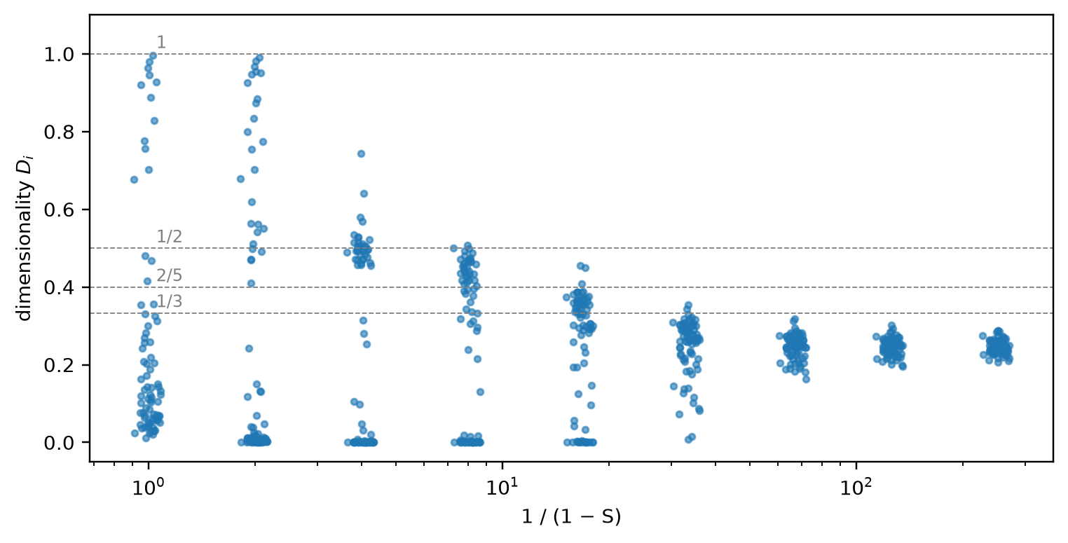
Scaling up the counts shows the paper's most striking observation: the amount of bottleneck
each feature gets, $D_i$, does not vary continuously with sparsity but jumps between a few
discrete values that correspond to regular geometric arrangements.
```{python}
#| code-summary: "Train n=80, m=20 across many sparsity values and scatter D_i"
#| fig-cap: "Dimensionality per feature against $1/(1-S)$ (log scale). Each point is one feature. Values pile up at 1 (own axis), 1/2 (antipodal pair), and fractions like 2/5 and 1/3 that correspond to pentagons and triangles in sub-spaces of the bottleneck. Dropped features sit at 0."
n, m = 80, 20
S_list = [0.0, 0.5, 0.75, 0.875, 0.94, 0.97, 0.985, 0.992, 0.996]
fig, ax = plt.subplots(figsize=(7, 3.6))
for S in S_list:
    W = fit_tms(n, m, S, steps=4000, importance_decay=0.97, seed=2).W
    D = feature_dimensionality(W)
    x = 1/(1-S) * (1 + 0.04*np.random.default_rng(0).standard_normal(n))
    ax.scatter(x, D, s=8, alpha=0.6, color="C0")
for y, lab in [(1, "1"), (0.5, "1/2"), (0.4, "2/5"), (1/3, "1/3")]:
    ax.axhline(y, color="gray", lw=0.6, ls="--"); ax.text(1.05, y+0.015, lab, fontsize=8, color="gray")
ax.set_xscale("log"); ax.set_xlabel("1 / (1 − S)"); ax.set_ylabel("dimensionality $D_i$")
ax.set_ylim(-0.05, 1.1)
plt.tight_layout()
```
At low sparsity the features split cleanly between "own axis" ($D_i = 1$), "antipodal pair"
($D_i = \tfrac12$) and "dropped" ($D_i = 0$). As sparsity rises the represented features move
to lower plateaus and eventually, when every feature is represented, settle near
$m/n = 0.25$, the uniform share. The paper's figure, with $n = 400$ features and $m = 30$
dimensions and much longer training, resolves more of the intermediate plateaus (2/5 for
pentagons, 1/3 for triangles and so on) than this quick run does. The plateaus are what the
paper means by **phase changes**: as sparsity increases, the optimal arrangement jumps
discretely from one polytope to another. A physicist will recognise this as a continuous
control parameter selecting among discrete symmetric configurations. It is a genuine and
robust result and the essay does not dispute it.
## 5. The essay's modification: correlated inputs plus hidden neurons
Now the part the essay added. Its appendix says: *"When we put correlated inputs and hidden
neurons in one model, related inputs grew onto the neurons. Making inputs fire more often
pushed the toy toward what the paper calls 'PCA-like' solutions, combining related inputs
into shared representations."*
Two changes to the toy.
1. **Correlated data.** Instead of independent features, 20 inputs are arranged in 4 groups of
5. A whole group turns on together with probability $p$; within an active group each
member gets an independent amplitude. This is the toy version of "in real data almost
nothing is related to nothing".
2. **A hidden layer.** After the 5-dimensional bottleneck there is a layer of $k$ ReLU
neurons before the output: $a = \mathrm{ReLU}(V h + c)$, $\hat x = U a + b$. These are the
"neurons" whose cleanliness we can now ask about; the original toy has none.
```{python}
#| code-summary: "Train the grouped model, sparse and dense"
n_groups, group_size, m, k = 4, 5, 5, 10
n = n_groups * group_size
group_of = np.repeat(np.arange(n_groups), group_size)

def fit_grouped(p_group, hidden=True, seed=0, steps=5000):
    gen = torch.Generator().manual_seed(seed)
    model = TMSHidden(n, m, k, gen) if hidden else TMS(n, m, gen)
    sampler = lambda b, g: sample_grouped(b, n_groups, group_size, p_group, g)
    train(model, sampler, None, steps=steps, seed=seed)
    return model

runs = {("sparse", True): fit_grouped(0.05, True),
        ("dense",  True): fit_grouped(0.50, True),
        ("sparse", False): fit_grouped(0.05, False),
        ("dense",  False): fit_grouped(0.50, False)}
```
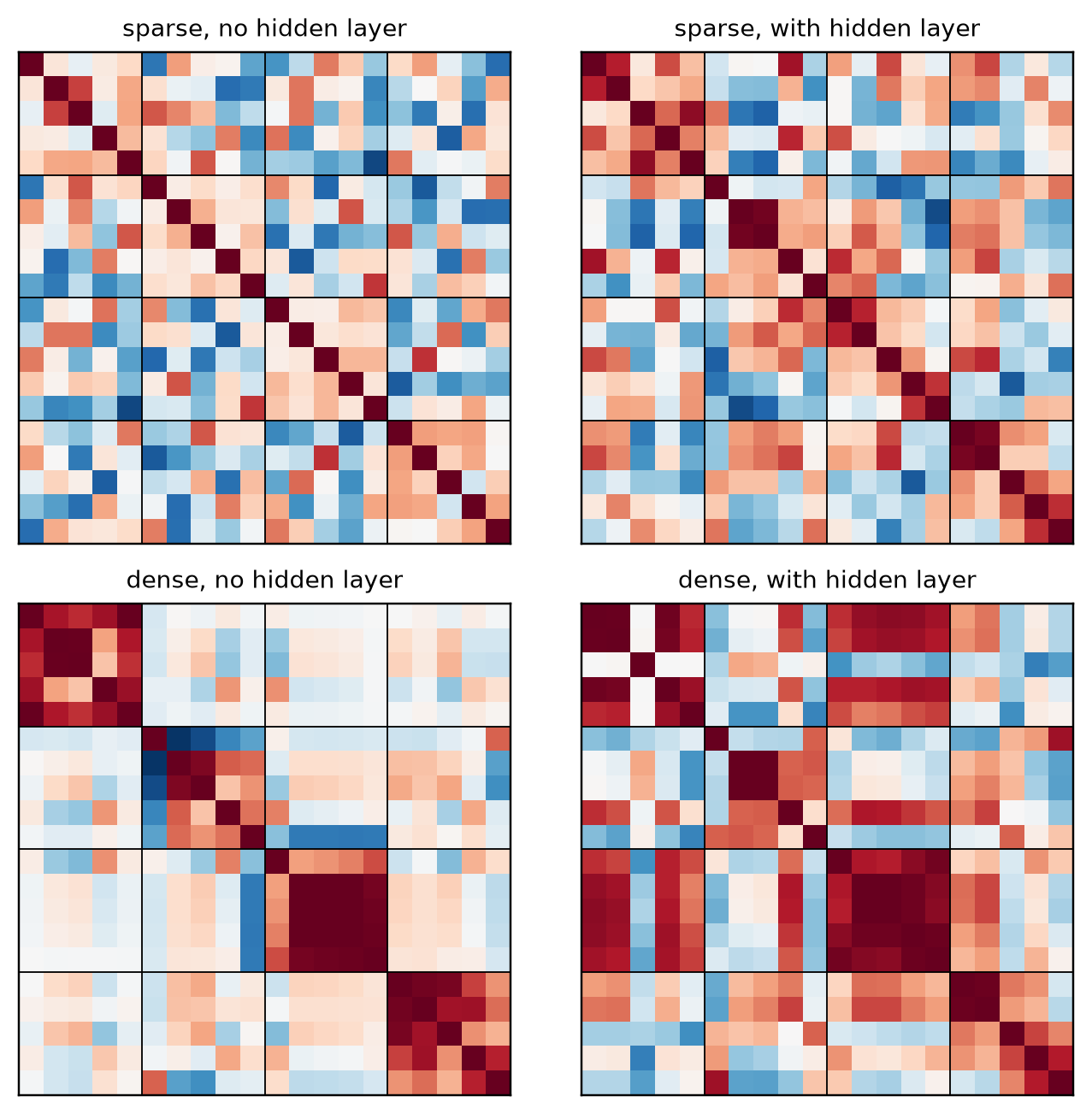
First, what the bottleneck does with correlated inputs. The cosine matrix between the 20
input directions $W_i$ shows whether the model gave each group a shared direction.
```{python}
#| code-summary: "Cosine between input directions"
#| fig-cap: "Cosine similarity between the bottleneck directions $W_i$ of the 20 inputs, which come in 4 correlated groups of 5 (block boundaries drawn). Left pair: original toy with no hidden layer. Right pair: with a hidden layer. Rows: groups rarely on (sparse) and often on (dense)."
fig, axes = plt.subplots(2, 2, figsize=(6.2, 6))
for r, regime in enumerate(["sparse", "dense"]):
    for c, hidden in enumerate([False, True]):
        W = runs[(regime, hidden)].W
        C = cosine_matrix(W)
        ax = axes[r, c]
        ax.imshow(C, cmap="RdBu_r", vmin=-1, vmax=1)
        for gb in range(group_size, n, group_size):
            ax.axhline(gb-0.5, color="k", lw=0.6); ax.axvline(gb-0.5, color="k", lw=0.6)
        ax.set_xticks([]); ax.set_yticks([])
        ax.set_title(f"{regime}, {'with' if hidden else 'no'} hidden layer", fontsize=9)
plt.tight_layout()
```
Reading the figure. Without a hidden layer (left column) the toy behaves as the paper
says: sparse groups are packed input by input, with no block structure, exactly as if the
inputs were independent; dense groups get the "PCA-like" solution in which each group of five
shares one direction. With a hidden layer (right column) the block structure appears *even
in the sparse regime*: related inputs are written to a shared direction and the hidden
neurons read that direction. That is the essay's "related inputs grew onto the neurons".
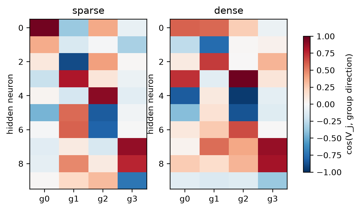
Second, what the hidden neurons read. For each hidden neuron $j$ we take the cosine of its
read direction $V_j$ with each of the four group directions, defined as the mean of each
group's $W_i$. The sign matters: a neuron that is positive on one group and negative on
another is a *contrast* between two things, which is what the essay calls a gate with two
poles, not a mixture.
```{python}
#| code-summary: "Hidden neurons in the group basis"
#| fig-cap: "Each row is one hidden neuron; each column a group of correlated inputs. Colour is the cosine between the neuron's read direction $V_j$ and that group's shared direction. Left: sparse groups. Right: dense groups. A neuron 'about' one group is a single strong cell; a contrast neuron has one red and one blue cell."
def group_cosines(model):
    W = model.W.detach(); V = model.V.detach()
    G = torch.stack([W[:, group_of == g].mean(1) for g in range(n_groups)], 1)  # (m, n_groups)
    G = G / G.norm(dim=0, keepdim=True)
    Vn = V / V.norm(dim=1, keepdim=True).clamp_min(1e-8)
    return (Vn @ G).numpy()

fig, axes = plt.subplots(1, 2, figsize=(6.4, 3.4))
for ax, regime in zip(axes, ["sparse", "dense"]):
    cs = group_cosines(runs[(regime, True)])
    order = np.lexsort((-np.abs(cs).max(1), np.abs(cs).argmax(1)))
    im = ax.imshow(cs[order], cmap="RdBu_r", vmin=-1, vmax=1, aspect="auto")
    ax.set_xticks(range(n_groups)); ax.set_xticklabels([f"g{g}" for g in range(n_groups)])
    ax.set_ylabel("hidden neuron"); ax.set_title(regime)
plt.colorbar(im, ax=axes, shrink=0.8, label="cos(V_j, group direction)")
```
::: {.beyond-inline}
The pole-by-pole audit of the hidden neurons that follows is our own analysis. The essay's
figure for this variant shows only the bottleneck's cosine structure.
:::
Because the output ReLU discards a neuron's negative side, what the neuron *transmits* is its
positive pole. So the fair question, in the essay's own terms, is whether the positive pole
is about one group. We count a neuron as "one group on the positive pole" if, among the
groups it reads with positive sign, one carries more than 80% of the positive weight; we
also record whether it has a strong negative pole on some other group.
```{python}
#| code-summary: "Summary over several seeds"
def classify(model):
    cs = group_cosines(model); V = model.V.detach()
    alive = (V.norm(dim=1) > 1e-2).numpy()
    pos = np.clip(cs, 0, None) ** 2
    share = pos.max(1) / np.maximum(pos.sum(1), 1e-8)
    return alive, share > 0.8, cs.min(1) < -0.5

print(f"{'regime':8s} {'alive':>6s} {'one-group +pole':>16s} {'…with strong -pole':>19s} {'mixed +pole':>12s}   (5 seeds x {k} neurons)")
for regime, p in [("sparse", 0.05), ("dense", 0.5)]:
    tot = np.zeros(4)
    for seed in range(5):
        alive, one, neg = classify(fit_grouped(p, True, seed=seed, steps=4000))
        tot += [alive.sum(), (one & alive).sum(), (one & neg & alive).sum(), (~one & alive).sum()]
    print(f"{regime:8s} {tot[0]:6.0f} {tot[1]:16.0f} {tot[2]:19.0f} {tot[3]:12.0f}")
```
The result is intermediate, and worth stating plainly rather than rounding toward either
side. Roughly three in five hidden neurons in the sparse regime, and about half in the dense
regime, have a positive pole that is about one group; a third of those also carry a strong
negative pole on another group, which is the "V versus O" structure the essay describes. The
remaining neurons read a positive combination of two groups. No neuron reads all four.
Widening the hidden layer to 20 neurons does not change the proportions. (Making the groups
fire more often makes the *bottleneck* more PCA-like, as the essay says, but it does not make
the hidden neurons cleaner in this count.)
One caution on reading this. The groups here are independent of each other, so a neuron
reading two groups *is* a mixture of unrelated things in the essay's sense. Adding
correlations and a hidden layer makes the bottleneck organise by group and gives many
neurons a one-group positive pole, but it does not make mixed neurons disappear. Whether real
networks are in a regime where two-group neurons are rare is exactly what the rest of the
essay tries to show empirically, and it is not something a toy can settle.
::: {.beyond}
## 6. Adding the missing benefit: readers instead of reconstruction
Section 5 put the relatedness into the *data*. But in a toy with independent inputs there is
nothing intrinsically related about any two of them: every partition into groups is a
relabelling of every other. So any grouping we saw there could be credited to the input
statistics. The essay's argument is about something else: a representation matters only
through what reads it, and sharing a direction between two inputs is a benefit when
downstream readers want them together. The original toy has no readers, so that benefit is
priced at zero. Here we put readers in and leave the inputs exactly as in the original toy:
independent and sparse.
**The setup.** The bottleneck $h = Wx$ feeds a hidden ReLU layer, which feeds $T = 12$ output
tasks. Every task has the same form: a rectified sum over five inputs,
$y_t = \mathrm{ReLU}\big(\sum_{i \in S_t} x_i - \theta_t\big)$, with $\theta_t$ cycling
through three thresholds. The only thing we vary is **how many distinct subsets $S_t$ the
twelve tasks factor through**, which we call $J$:
- $J = 4$: four disjoint subsets, each read by three tasks. A four-dimensional intermediate
(the four sums) serves every reader. This is maximal reuse.
- $J = 12$: twelve subsets chosen to overlap as little as possible, each read by one task.
No shared intermediate helps anyone. This is the control.
- $J = 6, 8$ in between.
With $J = 4$ and only four tasks the two conditions would be identical, which is the
relabelling point again; the difference appears only when several readers want the same
combination. That is what the essay calls reuse, so $J$ is the quantity under test rather
than a proxy for it.
**What to measure**, without reference to any grouping the data does not contain:
the **participation ratio** of the singular values of $W$ (the effective number of bottleneck
dimensions in use), the mean |cosine| between input directions for pairs that **share a
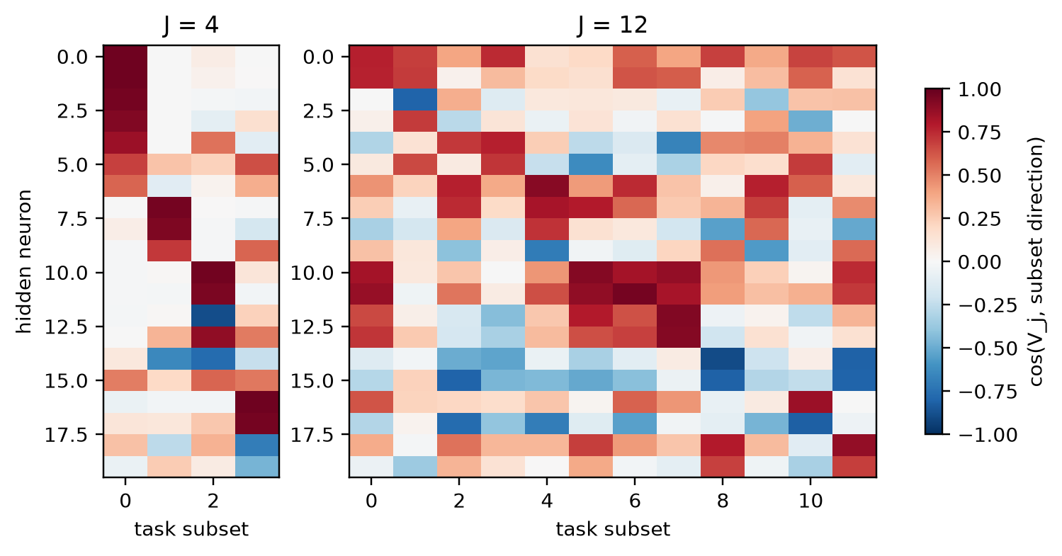
subset** versus pairs that **share none**, the **task loss**, and the hidden-neuron poles
scored against the task-defined subsets.
```{python}
#| code-summary: "Train the reader toy across the reuse knob J"
from common.toy_models import (ReaderToy, make_subsets, make_tasks, train_tasks,
                               participation_ratio, within_between_cosine)
n, m, k, T, fan, S_READ = 20, 5, 20, 12, 5, 0.9

def fit_readers(J, S=S_READ, seed=0, steps=4000, extra_tasks=()):
    subs = make_subsets(n, J, fan, seed=seed)
    tasks = make_tasks(subs, T) + list(extra_tasks(subs) if callable(extra_tasks) else extra_tasks)
    model = ReaderToy(n, m, k, len(tasks), torch.Generator().manual_seed(seed))
    L = train_tasks(model, tasks, n, S, steps=steps, seed=seed)
    return model, subs, tasks, L[-200:].mean()

Js = [4, 6, 8, 12]
reader_runs = {J: [fit_readers(J, seed=s) for s in range(2)] for J in Js}
print(f"{'J':>3s} {'max overlap':>12s} {'loss':>8s} {'PR':>6s} {'|cos| within':>13s} {'between':>8s}   (S = {S_READ}, 2 seeds)")
for J in Js:
    rows = []
    for model, subs, _, loss in reader_runs[J]:
        w, b = within_between_cosine(model.W, subs)
        rows.append((loss, participation_ratio(model.W), w, b))
    r = np.mean(rows, 0)
    subs = reader_runs[J][0][1]
    ov = max(len(set(a) & set(b)) for i, a in enumerate(subs) for b in subs[i+1:])
    print(f"{J:3d} {ov:12d} {r[0]:8.3f} {r[1]:6.2f} {r[2]:13.2f} {r[3]:8.2f}")
```
```{python}
#| code-summary: "Input directions, ordered by subset, at the two ends of the knob"
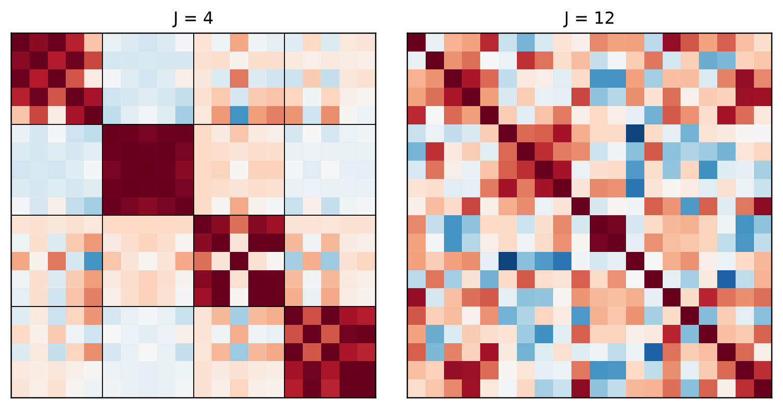
#| fig-cap: "Cosine between the bottleneck directions $W_i$ of the 20 independent inputs, ordered by the task subsets (boundaries drawn), for maximal reuse ($J=4$, left) and no reuse ($J=12$, right; inputs ordered by their first subset). The inputs are statistically identical in both panels; only the readers differ."
fig, axes = plt.subplots(1, 2, figsize=(7.2, 3.6))
for ax, J in zip(axes, [4, 12]):
    model, subs, _, _ = reader_runs[J][0]
    first = {}
    for j, s in enumerate(subs):
        for i in s: first.setdefault(i, j)
    order = sorted(range(n), key=lambda i: (first.get(i, 99), i))
    C = cosine_matrix(model.W)[np.ix_(order, order)]
    ax.imshow(C, cmap="RdBu_r", vmin=-1, vmax=1)
    if J == 4:
        for gb in range(fan, n, fan):
            ax.axhline(gb-0.5, color="k", lw=0.6); ax.axvline(gb-0.5, color="k", lw=0.6)
    ax.set_xticks([]); ax.set_yticks([]); ax.set_title(f"J = {J}")
plt.tight_layout()
```
With maximal reuse the bottleneck becomes four coarse directions, one per shared sum, with
the five inputs of each sum nearly parallel (|cosine| about 0.8 within, 0.2 between) and a
participation ratio of 4. Nothing about the inputs asked for this; the readers did. With no
reuse the same inputs are spread with no block structure, the participation ratio rises
toward 5, and the task loss is seventy times larger: twelve independent sums do not fit in
five dimensions, so the network packs them with interference. Intermediate $J$ gives
intermediate values of everything.
Two remarks on the control. First, it is the original toy's situation transposed up one
level: the quantities being packed are now the readers' sums rather than the inputs, but the
mechanism is the same. Second, the control is not a strawman. Each task still reads five
inputs through the same function; it just reads a combination nobody else wants.
```{python}
#| code-summary: "Hidden-neuron poles against the task subsets"
#| fig-cap: "Cosine between each hidden neuron's read direction and each subset's shared direction (the mean of its five $W_i$). Left: $J=4$, four subsets. Right: $J=12$, twelve subsets. With reuse, neurons are about one sum, some with a contrasting negative pole; without, they read many overlapping sums."
def subset_cosines(model, subs):
    W = model.W.detach(); V = model.V.detach()
    G = torch.stack([W[:, s].mean(1) for s in subs], 1); G = G / G.norm(dim=0, keepdim=True)
    Vn = V / V.norm(dim=1, keepdim=True).clamp_min(1e-8)
    return (Vn @ G).numpy()
fig, axes = plt.subplots(1, 2, figsize=(8, 3.6), gridspec_kw={"width_ratios": [4, 12]})
for ax, J in zip(axes, [4, 12]):
    model, subs, _, _ = reader_runs[J][0]
    cs = subset_cosines(model, subs)
    order = np.lexsort((-np.abs(cs).max(1), np.abs(cs).argmax(1)))
    im = ax.imshow(cs[order], cmap="RdBu_r", vmin=-1, vmax=1, aspect="auto")
    ax.set_xlabel("task subset"); ax.set_title(f"J = {J}")
axes[0].set_ylabel("hidden neuron")
plt.colorbar(im, ax=axes, shrink=0.8, label="cos(V_j, subset direction)")
```
```{python}
#| code-summary: "Does sparsity rescue the no-reuse control?"
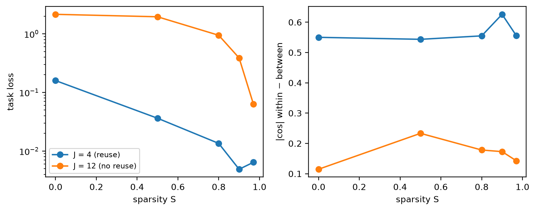
#| fig-cap: "Task loss (left) and the gap between within-subset and between-subset |cosine| (right) as a function of input sparsity, for maximal reuse and no reuse. Two seeds each."
S_list = [0.0, 0.5, 0.8, 0.9, 0.97]
curves = {J: [] for J in (4, 12)}
for Sp in S_list:
    for J in (4, 12):
        rows = []
        for s in range(2):
            model, subs, _, loss = fit_readers(J, S=Sp, seed=s)
            w, b = within_between_cosine(model.W, subs)
            rows.append((loss, w - b))
        curves[J].append(np.mean(rows, 0))
fig, axes = plt.subplots(1, 2, figsize=(8, 3.2))
for J, lab in [(4, "J = 4 (reuse)"), (12, "J = 12 (no reuse)")]:
    c = np.array(curves[J])
    axes[0].plot(S_list, c[:, 0], "o-", label=lab); axes[1].plot(S_list, c[:, 1], "o-", label=lab)
axes[0].set_yscale("log"); axes[0].set_xlabel("sparsity S"); axes[0].set_ylabel("task loss"); axes[0].legend(fontsize=8)
axes[1].set_xlabel("sparsity S"); axes[1].set_ylabel("|cos| within − between")
plt.tight_layout()
```
The reuse condition is clean and nearly lossless at every sparsity. The no-reuse condition
is simply infeasible when inputs are dense, and only approaches a low loss at very high
sparsity, where packing with interference becomes cheap. This is the original toy's
phase diagram again, now driven by the readers: superposition is what a network does when
the things it must represent are unrelated *to its readers* and rare enough to pack.
### A private offshoot
If reuse makes inputs coarse, what happens when one reader wants fine structure? We keep the
$J = 4$ tasks and add a single extra task that reads one input alone, $y = x_{i^\star}$ for
some $i^\star$ in the first subset. The prediction from the essay's picture is that
$W_{i^\star}$ stays aligned with its group direction and grows a private component that the
rest of the group lacks.
```{python}
#| code-summary: "One extra reader on a single input"
def offshoot_stats(extra, seeds=3):
    out = []
    for s in range(seeds):
        ex = (lambda subs: [([subs[0][0]], 0.0)]) if extra else ()
        model, subs, _, loss = fit_readers(4, seed=s, extra_tasks=ex)
        W = model.W.detach(); g = W[:, subs[0]].mean(1); g = g / g.norm()
        def split(i):
            w = W[:, i]; par = float(w @ g); return par, float((w - par * g).norm())
        t = split(subs[0][0]); o = np.mean([split(i) for i in subs[0][1:]], 0)
        out.append((loss, t[0], t[1], o[0], o[1]))
    return np.mean(out, 0)
print(f"{'extra reader':>13s} {'loss':>7s} {'target ∥ group':>15s} {'target ⊥':>9s} {'others ∥ group':>15s} {'others ⊥':>9s}")
for extra in (False, True):
    r = offshoot_stats(extra)
    print(f"{str(extra):>13s} {r[0]:7.3f} {r[1]:15.2f} {r[2]:9.2f} {r[3]:15.2f} {r[4]:9.2f}")
```
The single extra reader makes the target input's private component more than six times
larger while leaving its alignment with the group untouched, and leaves the other four members of the group as they
were. In the essay's language, the input has a group direction and an offshoot, and the
offshoot exists because something reads it. This is the smallest possible model of
"recursive generalisation": a coarse representation that grows a finer branch exactly where
a downstream reader needs one.
### What this adds to the picture
- The relatedness that makes a network group things is not in the inputs. It is in the
readers. Identical input statistics give clean coarse directions under shared readers and
packing under unshared ones.
- Superposition and generalisation are not two learning principles here; they are what one
objective does in two regimes of reader structure. Packing wins only when the quantities
readers need are unrelated to each other and sparse enough to overlap cheaply.
- What the toy cannot tell us is which regime a real network's readers are in. The essay's
bet is that in real data "almost nothing is related to nothing", so real readers are
overwhelmingly of the shared kind. That is the empirical claim the rest of the essay has
to carry.
:::
## 7. What to carry into the essay
- **Packing is real and robust in the toy's world.** Independent sparse features in a narrow
bottleneck with nothing downstream get packed into polytopes, with discrete phase changes.
- **Correlation plus a hidden layer changes the picture, partly.** Related inputs share
directions in the bottleneck, and about half to two thirds of hidden neurons have a
one-group positive pole, some with a contrasting negative pole. This is the mechanism the
essay calls generalisation, and it appears as soon as the toy has somewhere for related
things to grow. But a sizeable minority of neurons still read two unrelated groups, so the
toy supports the essay's mechanism without supporting its strong claim.
- **The toy cannot say which regime real networks are in.** That is an empirical question and
it is what the essay's vision and language experiments are for.
## 8. What the toy does and does not say
The toy's results are robust and the essay accepts them: when independent, sparse features
must be squeezed through a narrow linear bottleneck and reconstructed, the optimum packs
them into non-orthogonal polytopes, with discrete phase changes as sparsity varies.
The essay's objection is to three modelling choices that it argues do not hold in real
networks:
- **Features are given in advance** and independent. In a real network nothing is defined in
advance; everything is grown, and real data has structure at every scale ("a rare person
still has a country, a job and a name").
- **Nothing reads the representation.** The loss is reconstruction, so each feature is an end
in itself. In a real network a representation only matters through what downstream reads
it, and sharing a direction between *related* things is a benefit (reuse), not a cost.
- **There are no hidden neurons** in the main experiments. Superposition in the toy is about
directions in a bottleneck; reports of polysemanticity in real networks are about
mixtures in neurons. The paper itself studies hidden neurons and correlated features, but
separately.
The toy therefore predicts where to *expect* packing: memories that are ends in themselves
and related to nothing else. The essay's claim is that real networks are rarely in that
regime, and the rest of the essay is an attempt to show this empirically in vision and
language models.
::: {.beyond}
## Questions from the reading group
Raised in discussion on 22 October 2026. The answers are ours, not the essay's.
**What does the readers experiment in section 6 actually test? If the number of independent
tasks exceeds the bottleneck, isn't the network simply forced into something like
superposition?**
At the endpoints, yes, the outcome is forced by counting. Twelve independent sums cannot pass
losslessly through five dimensions, so the network must drop some or pack them with
interference; four sums can, so it does. The toy discovers nothing there.
What it tests is a claim that is often read into the original toy: that *more features than
dimensions implies superposition*. In both of our conditions there are twenty inputs and five
dimensions, and in both the inputs are independent and sparse, so the original toy's premise
holds identically. Yet with shared readers the network does not pack the twenty inputs at
all. It builds four coarse directions and discards the within-group identity that nobody
downstream asked for. The relevant count is not "features versus dimensions" but "what the
readers need versus dimensions", and when readers want shared things the answer is
coarse-and-clean rather than packed. That is the essay's "coarser, never fractured" in its
smallest form.
The non-trivial content is at the margins rather than the endpoints. With six or eight
distinct sums the required information exceeds the bottleneck but overlaps partially, and
the network's compromise is intermediate rather than a switch. When packing is forced, it only
becomes cheap at high sparsity, so the original phase boundary reappears for the readers'
quantities, which supports reading superposition as what one objective does in one regime
rather than as a second principle. And the offshoot test shows that a single reader is enough
to grow a private direction inside a coarse one.
A tighter version would hold the *dimension* of what readers need fixed and vary only its
*structure*: for instance eight tasks on subsets that overlap hierarchically against eight on
subsets that overlap at random. That would separate "how much information" from "how
organised the information is", which is closer to the essay's real claim. Not yet built.
:::
## Further reading
- Elhage et al., *Toy Models of Superposition* (2022), especially the sections on feature
geometry, phase diagrams, and correlated features.
- The essay's appendix sections "Toy Models" and "A Note on Features and Definitions".